以下のコードは、Code値を入力しsheet2て強調表示し、このマクロを実行すると機能します。
Selection.Offset(0, 1).FormulaR1C1 = "=IFERROR(VLOOKUP(RC[-1],Sheet1!C[-1]:C,2,FALSE),"""")"
Selection.Offset(0, 2).FormulaR1C1 = "=IFERROR(VLOOKUP(RC[-2],Sheet1!C[-2]:C,3,FALSE),"""")"
Selection.Offset(0, 1).Value = Selection.Offset(0, 1).Value
Selection.Offset(0, 2).Value = Selection.Offset(0, 2).Value
編集:入力時に値を更新したい場合は、use(@PeterAlbertに最適化を追加していただきありがとうございます!):
Private Sub Worksheet_Change(ByVal Target As Range)

    'end if the user made a change to more than one cell at once?
    If Target.Count > 1 Then End

    'stop system activating worksheet_change event while changing the sheet
    Application.EnableEvents = False

    'continue if column 1(A) was updated
    'and
    'dont continue if header or row 1 was changed
    If Target.Column = 1 And Target.Row <> 1 Then

        With Target.Offset(0, 1) 'alter the next cell, current column +1 (column B)

            'RC1 = current row and column 1(A) e.g. if A2 was edited, RC1 = $B2
            'C1:C2 = $A:$B
            .FormulaR1C1 = "=IFERROR(VLOOKUP(RC1,Sheet1!C1:C2,2,FALSE),"""")"
            .Value = .Value 'store value
        End With

        With Target.Offset(0, 2) 'alter the next cell, current column +2 (column C)

            'C1:C3 = $A:$C
            .FormulaR1C1 = "=IFERROR(VLOOKUP(RC1,Sheet1!C1:C3,3,FALSE),"""")"
            .Value = .Value 'store value
        End With

    End If

    Application.EnableEvents = True 'reset system events
End Sub
RCの説明:
数式のFormulaR1C1種類は、現在のセルを基準にしてセルを参照するときに使用すると便利です。覚えておくべきいくつかのルールがあります:
Rは行を表し、列を表し、その後Cの整数があれば、行または列を定義します。- 基礎として、
RC式はそれ自体を参照します。
Rまたはに続く数字Cは[]、それ自体へのオフセットです。たとえば、セル内A1にいて使用するR[1]C[1]場合は、セルを参照しB2ます。Rまた、とに続く任意の数字Cは正確です。たとえば、現在のセルに関係なく参照する場合は、 ;R2C2も指します。B2と
C5セル内にいる場合、たとえば次のように使用Range("C5").FormulaR1C1 =してコーディングすると、事態が複雑になります。
"=RC[-1]"参照セルB5"=RC1"セルを参照A5し、より正確に$A5"=R[1]C[-2]"参照セルA6"=Sum(C[-1]:C5)"です=Sum(B:E)、もっと正しく=Sum(B:$E)