他の人が述べたように、信号の周波数を誤解しています。いくつかのことを明確にするために例を挙げましょう。
Fs = 200;                        %# sampling rate
t = 0:1/Fs:1-1/Fs;               %# time vector of 1 second
f = 6;                           %# frequency of signal
x = 0.44*sin(2*pi*f*t);          %# sine wave

N = length(x);                   %# length of signal
nfft = N;                        %# n-point DFT, by default nfft=length(x)
                                 %# (Note: it is faster if nfft is a power of 2)
X = abs(fft(x,nfft)).^2 / nfft;  %# square of the magnitude of FFT

cutOff = ceil((nfft+1)/2);       %# nyquist frequency
X = X(1:cutOff);                 %# FFT is symmetric, take first half
X(2:end -1) = 2 * X(2:end -1);   %# compensate for the energy of the other half
fr = (0:cutOff-1)*Fs/nfft;       %# frequency vector

subplot(211), plot(t, x)
title('Signal (Time Domain)')
xlabel('Time (sec)'), ylabel('Amplitude')

subplot(212), stem(fr, X)
title('Power Spectrum (Frequency Domain)')
xlabel('Frequency (Hz)'), ylabel('Power')

これで、FFT のピークが 6Hz の信号の元の周波数に対応することがわかります。
[v idx] = max(X);
fr(idx)
ans =
      6
Parseval の定理が成り立つことも確認できます。
( sum(x.^2) - sum(X) )/nfft < 1e-6
オプション 2
または、信号処理ツールボックスの関数を使用できます。
%# estimate the power spectral density (PSD) using the periodogram
h = spectrum.periodogram;
hopts = psdopts(h);
set(hopts, 'Fs',Fs, 'NFFT',nfft, 'SpectrumType','onesided')

hpsd = psd(h, x, hopts);
figure, plot(hpsd)

Pxx = hpsd.Data;
fr = hpsd.Frequencies;
[v idx]= max(Pxx)
fr(idx)

avgpower(hpsd)

この関数は対数スケールを使用することに注意してくださいplot(fr,10*log10(Pxx)):plot(fr,Pxx)